
Abstract
Intrusion Detection System (IDS) predominantly works for detecting malicious attacks to computer network. In this project, we propose some IDS models based on Artificial Neural Network and clustering techniques. ANNs can only be built if there is availability of an effective dataset. A dataset with a sizable amount of quality data which mimics the real world, can help to train and test an intrusion detection system. We will introduce the NSL-KDD dataset. It has been used to study the effectiveness of the neural network-based classification algorithm to detect anomalies in the network traffic patterns. The entire analysis has been conducted using Matlab.
Keywords – Intrusion Detection System, Artificial Neural Network, NSL-KDD dataset.
1. Introduction
Firewalls represent the most widely used security mechanisms in corporate networks but they can only protect from outside intruders. Hence, it is very important to have additional protection mechanisms in the internal host and network to prevent unauthorized access and possible inside threats. A key activity is called Intrusion Detection and consists of monitoring a system or a network. Intrusion Detection Systems – briefly IDSs – fulfill such a purpose by breaking intrusive behaviors and consequently informing the security specialists.
In practical way, it is not possible to provide a complete prevention. However, it is viable to detect these intrusion attempts so that some actions may be taken to repair the damage. IDS goal is to identify unauthorized activity by inspecting individual machines and/or inbound network traffic. They are also important in order to understand new attacks and how they work so that an immediate response can be taken to prevent similar attacks. Snort is an example of a well-known IDS product available for several platforms including Windows, Linux and MAC.
Despite, there are two types of IDSs: Network Based and Host Based, in this project we’ll address only the Network Based IDS.
1.1. Objective
Our objective is to build an IDS model in order to separate safe connections from threats. We used IDS systems with Artificial Neural Networks – ANNs – in order to classify possible malicious activities with high accuracy and once incorrectly classifying some data, they learnt from their own mistakes and improve their efficiency. We also made comparison with a clustering algorithm to see how well they perform with zero-day attacks.
The rest of this project is organized as follows: Section II presents the state-of-the-art. Section III reports the employed classification techniques. Section IV shows the key activities to create the model. Final results and tests are depicted in section V, with conclusions reported in section VI.
2. State-of-the-art
Network-based IDS systems detect attacks by capturing and analyzing network packets, from sensors placed at various points in a network. In general, there are two primary models to analyzing events to detect attacks: misuse detection and anomaly detection. In misuse detection model IDS detect intrusions by looking for activity that corresponds to known signatures of intrusions or vulnerabilities. Anomaly detection instead, detects intrusions by searching abnormal network traffic and they have the ability to detect symptoms of attacks without specifying model of attacks. We want to work on this second class of detection (anomaly detection).
The majority of tools available today refer to the misuse detection model, meaning that administrators need to regularly update vulnerabilities database. Instead, commercial tools available for anomaly detection have limitations in detecting real intrusions, and Neural Network is a efficient way to improve the performances of these IDS systems. Applying the Neural Network approach to Intrusion Detection, we first have to expose NN to normal data and to attacks to automatically adjust coefficients of the NN during the training phase. Performance tests are then conducted with real network traffic and attacks.
3. Employed classification techniques
In this section we briefly review the data mining techniques that are employed in our models to evaluate performances and make comparisons.
Feedforward Neural Network. They consist of a series of layers. The first layer has a connection from the network input. Each subsequent layer has a connection from the previous layer. The final layer produces the network’s output. A feedforward network with enough neurons in the hidden layers, can fit any finite input-output mapping problem.
Radial basis function. Similarly to the previous one, they consist of two layers. A hidden radial basis layer and an output linear layer. The transfer function is described by a radial basis function with its maximum to 1 when the input is 0.
Clustering Technique. Clustering data is an excellent application for neural networks. This process involves grouping data by similarity. Self-organizing maps algorithm is a unique method in that it combines the goals of the projection and clustering algorithms. It can be used at the same time to visualize the clusters in a dataset, and to present the set on a two dimensional map.
4. Methodology
Let us focus on the implementation of the model. The IDS system proposed in this work is the result of several key activities depicted in figure 1.
1. Dataset. The dataset used for training the model is known as NSL-KDD, which is provided by DARPA. It is a refined version of its predecessor and it has been widely used for simulating and testing the IDS systems. A second database containing new attack patterns has been used for testing. Each record is described by 42 attributes unfolding different features of the flow and a label assigned to each either as an attack type or as normal.
2. Pre-processing. To facilitate the analysis, the whole dataset has been split by two. In one side the input matrix with the 41 attributes that characterize the connection; on the other hand the target matrix which contains only the labels.
3. Codification. Neural network works best only on numerical data, which requires conversion of the textual data in the dataset to a numerical value. For this reason, the variables ‘protocol type’, ‘service’, ‘flag’ and ‘label’ need to be converted into numerical values. The attack classes are mapped with a 5 digits and constitutes the output value. The other attributes are simply mapped with numerical values in a range from 1 to 81.
| Type of attribute | Attribute | Mapping |
|---|---|---|
| Label | Normal | 10000 |
| DoS | 01000 | |
| Probe | 00100 | |
| R2L | 00010 | |
| U2R | 00001 | |
| Protocol type | TCP | 1 |
| UDP | 2 | |
| ICMP | 3 | |
| Flag | All flags | 5 to 15 |
| Service | All services | 16 to 81 |
The whole mapping process took almost 45 minutes.
4. Normalization. In ANN we need to normalize the inputs, otherwise the network will be ill-conditioned. It is done to have the same range of values for each of the inputs to the ANN model. This can guarantee stable convergence of weight and biases.
5. Features selection. High dimensional data are very common in network sniffing due to the multiple features that the sniffer is able to capture. These attributes are not always convenient and one approach is to reduce the dimension of the feature space using a well-suited technique namely Principal Component Analysis (PCA). Its outcome is to project a feature space onto a smaller subspace. By selecting the most important features – called principal components – we improved performances and saved computational time. Thus, the final dataset undergo a dimensionality reduction and contains 15 features.
6. Classification techniques. For the analysis, Matlab 2018a v9.4.0 has been used with the integrated Neural Network toolbox for pattern recognition. The system is a CPU Intel Core i5 @1.7GHz and 8GB of RAM. The operating system is a Microsoft Windows 10 Enterprise edition. The tests have been conducted employing a feedforward neural network, a RBF network and a clustering technique. K-fold Cross-validation has been adopted.
7. Intrusion detection evaluation. In this project, we consider the Detection rate (DR) as principal metric. This parameter is mostly adopted in literature. To compare results, we also used the Accuracy rate and Precision rate.
5. Experiments & Results
Let’s talk more in detail about the dataset and the results that we obtained from the trained IDS models. Some experiments are proposed with the aim to provide the optimal solution for the classification problem.
5.1. Dataset
NSL-KDD is a public dataset created in 2007 by sniffing packets during a day-by-day network activity. The simulation network was made of a factitious military network consisting of three target machines running various operating systems and services. Additional three machines were then used to spoof different IP addresses to generate traffic. Finally, a sniffer recorded all network traffic using the TCP dump format. The total simulated period was seven weeks.
It can be considered as a representative of an existing real world scenario. Furthermore, the number of records is reasonable and makes it affordable to run the experiments on the complete set without the need to randomly select a small portion. Each record represents a connection intercepted through the network, with 41 attributes to describe it and a label assigned to each either as a specific type of attack or as normal.
Each pattern of the NSL-KDD dataset falls into any of the following classes, namely, Normal and four different kinds of attacks such as Probe, Denial of Service (DoS), Remote to Local (R2L) and User to Root (U2R):
- DoS Attack. Attacks which attempt to crash the victim host by exhausting its computing or memory resources, so it cannot handle legitimate requests.
- Probe Attack. Attacks scanning computer networks to gather information or find known vulnerabilities, which are exploited for further or future attacks.
- R2L Attack. Attacks in which an unauthorized user can gain local access through bypassing normal authentication and executing commands on the victim machine.
- U2R Attack. Attacks in which a normal user with login access can gain the privileges of root users by bypassing normal authentications.
5.1.1. Distribution of class label
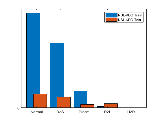
Two databases have been employed as part of the NSL-KDD packet. One for training and testing the model on known attacks using the k-folds cross validation and a second one employed solely to test the model’s behavior on unknown attacks. NSL-KDD Train contains 24 different attack patterns plus the normal connections; in contrast the NSL-KDD Test consists of 37 different attack patterns and the normal connections. The second database is therefore used to categorize attacks that have never been seen before.
| Type of connection | NSL-KDD Train | NSL-KDD Test |
|---|---|---|
| Normal | 67,343 | 9,711 |
| DoS | 45,927 | 7,460 |
| Probe | 11,656 | 2,421 |
| R2L | 995 | 2,885 |
| U2R | 52 | 67 |
| Total | 125,973 | 22,544 |
The total amount of zero-day attacks enclosed in the Test database is 3,752 and it constitutes the 30% of the database patterns. All the patterns for both databases fall into 5 main classes. They contain some low frequency attack classes like R2L and U2R. As a result the neural network may not use these instances during the training process. This is exactly what we expect to have in a real scenario because some types of threats like DoS and DDoS are more likely to happen than others.
5.2. Training and Testing
The train dataset was split into 10 non duplicated subsets and any nine of the subsets will be used for training the model and the remaining one for testing. This is termed as 10-fold cross validation.
5.2.1. PCA Analysis
Before applying any neural network models, PCA analysis was first employed to the original data to explore possibilities for data reduction in further predictions. We want to demonstrate that a combination between PCA and the ANN performs well even if a few axes are considered to represent the records.
PCA analysis was executed according to the various situations. The five principal components having a cumulative variation of more than 90% are retained and the others were tested to seek the optimal number of axes.
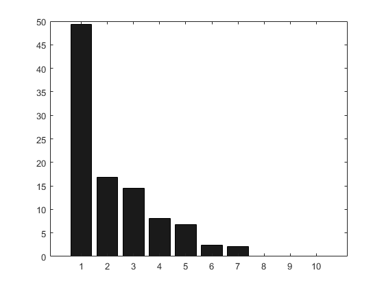
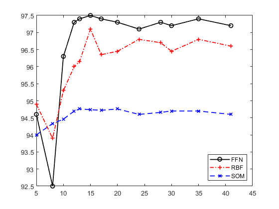
Using the classification techniques, we experimented the dataset on a new feature space generated by several PCA’s axes. We performed the different experiments considering 5, 8, 10, ..., 41 axes, because the cumulative variation with 5 axes is already more than 90%. For every neural network there is not much difference in the accuracy rate considering more than thirteen axes; that is where the graph becomes flat. The result shows that 15 axes are slightly better than any other. In general using fifteen axes, we obtain a higher accuracy than we would have using the entire database. In addition, the computation time is reduced by a factor of approximately three when considering 15 principal components. Hence, it is better to reduce the space on which the connection records are represented before applying any learners.
5.2.2. Feedforward with PCA
To evaluate the performance of the employed feedforward network, experiments varying the number of neurons in the hidden layer were conducted. Increasing the number of neurons increases as well the demand for computational capacity and the overfitting occurrence. The network was trained for 100 epochs. The best performance was obtained using 8 neurons, although the R2L detection rate was always under 10% for every model. Furthermore, increasing the number of neurons produced some overfitting occurrences.
| Detection rate | FFN-2N | FFN-8N | FFN-12N | FFN-20N |
|---|---|---|---|---|
| Hidden layer | 2 | 8 | 12 | 20 |
| Time | 5’30” | 6’20” | 15’10” | 30’30” |
| Normal | 85.0% | 99.1% | 99.0% | 98.9% |
| DoS | 88.1% | 98.3% | 97.4% | 97.3% |
| Probe | 78.8% | 93.2% | 93.7% | 94.3% |
| R2L | 0.0% | 7.7% | 6.2% | 7.4% |
| U2R | 0% | 0% | 0% | 0% |
| Accuracy | 84.85% | 97.51% | 97.22% | 97.10% |
| DR | 83.56% | 98.98% | 98.85% | 98.73% |
The confusion matrix for the proposed model with 8 neurons reports an overall accuracy of 97.5%. The minimum accuracy of the classification has been observed for class 5 (U2R), which is 0%, probably due to the reduced amount of samples currently in the database for this pattern. The false positive rate – 0.46% – is lower than false negative – 1.86%. In general, a false negative is the most dangerous state since the security professional has no idea that an attack took place.
| Normal | DoS | Probe | R2L | U2R | Total % | |
|---|---|---|---|---|---|---|
| Normal | 66,768 | 756 | 640 | 904 | 51 | 96.6 |
| DoS | 221 | 45,125 | 135 | 11 | 0 | 99.2 |
| Probe | 333 | 46 | 10,866 | 3 | 1 | 96.6 |
| R2L | 21 | 0 | 15 | 77 | 1 | 68.1 |
| U2R | 0 | 0 | 0 | 0 | 0 | 0 |
| Total % | 99.1 | 98.3 | 93.2 | 7.7 | 0 | 97.5 |
5.2.3. RBF with PCA
We design a two-layer network, setting the goal for the MSE to 0.01 and the radial function’s spread to 10. We didn’t notice any significant performance improvement by changing the function’s spread. The larger spread is, the smoother the function approximation. Too large a spread means a lot of neurons are required to fit a fast-changing function. Too small a spread means many neurons are required to fit a smooth function, and the network might not generalize well.
During the training process the network increases the number of neurons by 50 each round until the mean squared error falls below the goal. This analysis is greedy of memory, so we have randomly selected the 10% of the records producing a smaller database of 12,597 patterns. From the confusion matrix, we see a false positive rate – 2.14% – greater than the false negative – 0.58%.
| Normal | DoS | Probe | R2L | U2R | Total % | |
|---|---|---|---|---|---|---|
| Normal | 6,674 | 23 | 43 | 6 | 0 | 98.9 |
| DoS | 135 | 4,483 | 8 | 0 | 0 | 96.9 |
| Probe | 54 | 31 | 1,033 | 1 | 0 | 92.3 |
| R2L | 72 | 0 | 0 | 26 | 0 | 26.5 |
| U2R | 8 | 0 | 0 | 0 | 0 | 0 |
| Total % | 96.1 | 98.8 | 95.3 | 78.8 | 0 | 96.9 |
5.2.4. Self-organizing maps with PCA
We employed a 20x20 Kohonen’s Self Organizing Map with an hexagonal topology to build a two dimensional map of patterns. We trained the network for 50 epochs.
Assigning Labels. To assign labels to SOM neurons we maintain a hit score matrix h(i, j) where i is the class label index and j is the neuron index. As neuron j gets selected as winning neuron for more input samples from class i, h(i, j) score increases. After the SOM is trained, inputs from the training set are presented to determine the winning neurons. Hits score of the winning neuron for the given label is ranked assigning a higher score to a neuron that is closer to the input pattern in terms of Euclidean distance. Neurons are labeled with the class label, which has the highest hit score.
Pattern visualization. To visualize the cluster structure, a graphic display called U-Matrix is used. It shows the distances between weight vectors of the neurons using a color scale. The darker colors represent larger distances, and the lighter colors represent smaller distances.
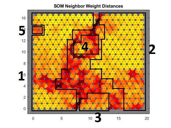
Figure 6 shows the U-Matrix of the SOM with assigned labels. It is important to note that patterns can be assigned neurons on different regions of the SOM since different stages of a connection can exhibit different behavior. Analysis of the U-Matrix reveals that five regions emerge from the SOM: from left (Region 1), right (Region 2), lower (Region 3), center (Region 4) and upper left (Region 5). Region 1, which is the larger Region, contains normal packets with the connections that are not classified as risky. Region 2 contains denial of service attacks where the attacker sends spoofed SYN packets. Region 3 and 4 are respectively Probe and R2L attacks. Finally the smaller area, that is very though to find, the User to Root attacks which have only 52 samples.
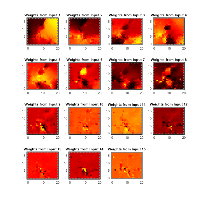
Probe and denial of service attacks are commonly clustered together. This is due to the fact that both type of attacks have observable impacts on network traffic. Accuracy implies the recognition of a pattern based on a given input to the SOM. From the analysis, we noticed that the U2R attack type still remains undetected. The overall model’s accuracy rate is 95.2%.
| Normal | DoS | Probe | R2L | U2R | Total % | |
|---|---|---|---|---|---|---|
| Normal | 65,299 | 702 | 475 | 361 | 41 | 97.6 |
| DoS | 782 | 44,549 | 1,758 | 0 | 0 | 94.6 |
| Probe | 1,018 | 659 | 9,414 | 16 | 1 | 84.7 |
| R2L | 244 | 17 | 9 | 618 | 10 | 68.8 |
| U2R | 0 | 0 | 0 | 0 | 0 | 0 |
| Total % | 97.0 | 97.0 | 80.8 | 62.1 | 0 | 95.2 |
5.2.5. Analogies between models
The comparison between the three different models changing the number of axes used for the test shows that the feedforward network gave the best performances. The other two networks never reached this level of accuracy but for both of them the shape of the curve is similar. In general considering the overall accuracy as the only metric, the RBF network behaves better than SOM but worse than feedforward network.
The best threats detection is reached with the RBF network, while feedforward got the best overall detection rate. Examining the false alarm rate, the RBF model could be considered in relation to the low number of false negative alarms. A false positive alarm can be mitigated using a double check, for example using a host-based IDS; in contrast, false negative cannot.
| Detection rate % | FFN | RBF | SOM |
|---|---|---|---|
| Time | 6’20” | 90’ | 83’ |
| Normal | 99.1 | 96.1 | 97.0 |
| DoS | 98.3 | 98.8 | 97.0 |
| Probe | 93.2 | 95.3 | 80.8 |
| R2L | 7.7 | 78.8 | 62.1 |
| U2R | 0 | 0 | 0 |
| Accuracy | 97.51 | 96.98 | 95.2 |
| DR | 98.98 | 95.37 | 96.54 |
| Precision | 95.99 | 98.73 | 97.31 |
5.2.6. Zero-day attacks
We want to test our employed models on a new class of patterns to see how well they perform with zero-day attacks. The test database contains known and unknown patterns as specified in section 5.1.1. In order to determine the best model as possible, we retrained our neural networks on the entire train database; so this time, cross validation hasn’t been adopted.
The ability of our models to detect the right class for R2L and U2R attack types was very low, so we kept the analysis on a higher level, focusing on the system’s ability to discriminate between normal connections (safe) and threats. If the IDS is able to split between safe and unsafe means that a security specialist has a clue that an attack is taking place also if he/she doesn’t realize which kind of threat it is.
| Detection rate % | FFN | RBF | SOM |
|---|---|---|---|
| Normal | 93.0 | 88.7 | 96.7 |
| Attack | 75.1 | 77.5 | 64.7 |
| False positive | 3.0 | 4.9 | 1.4 |
| False negative | 14.2 | 12.8 | 20.1 |
| Accuracy | 82.80 | 82.30 | 78.50 |
| DR | 93.50 | 90.10 | 96.30 |
The main drawback which persists in combining these algorithms with PCA is the poor prediction ratio rate of the R2L class which is in most of the time classified as normal. This is due to its low presence in the training dataset (0.23%). The testing dataset has three times the number of R2L samples than the training dataset.
The next step was to isolate and test known and unknown attacks apart to measure the capability of the system to predict new patterns. The RBF employed model was able to detect new types of threats with a detection rate of 75.1%. Unfortunately nobody gave reasonably good performances trying to discriminate the 4 attack classes. In fact only 35% of the samples were correctly classified in one of the 4 threat classes. However, R2L and U2R attack types in the test dataset could not be detected by classification techniques. This suggests to perform other unsupervised machine learning or data mining algorithms to deal with these new attacks that should be detected as new attacks. In contrast, known attack detection rate is higher and again the RBF model performs best.
| Threats detection % | FFN | RBF | SOM |
|---|---|---|---|
| Zero-day attack | 70.9 | 75.1 | 44.7 |
| Known attack | 76.8 | 78.5 | 73.0 |
Relatively to SOM neural network the result showed that more information are needed to identify the specific attack pattern but it can provide an approximate identification using existing features. In general we are far away from the performances obtained during the first part of the analysis but it bodes well for the future.
5.2.7. Comparison with similar analysis
We report results of analogous works conducted using neural networks and other machine learning algorithms on the same dataset. The Canadian Institute for Cybersecurity reports that about 98% of the records in the train set and 86% of the records in the test set were correctly classified using 21 different learners on the NSL-KDD dataset.
| Accuracy % | Result |
|---|---|
| [2] SVM | 96.55 |
| [2] PCA + SVM | 99.70 |
| [4] Decision tree | 96.95 |
| [4] K-means clustering | 96.41 |
| [3] Feedforward | 95.05 |
6. Conclusions
This project proposed an IDS integrating Principal Components Analysis with three ANNs for supporting IDS systems. Dimensionality reduction using PCA removes noisy attributes and retains the optimal attribute subset. The obtained results show that the proposed models based on training data obtained from PCA are able to detect and classify, with high correct detection rate (average detection rate of 96%), normal and intrusion behaviors through connection parameters. The results suggest that IDS systems based on anomaly are in fact a great alternative to widespread IDS systems based on signature.
Excepting for the R2L and U2R attack types, which presented only low results in terms of accuracy rate, a low index of false negatives and false positives was still observed, which results an increase in the network manager productivity due to the decrease of false generated alarms analysis that would be required by the IDS system.
The main concern for IT System Administrators is related with the false negative. Though IDSs work properly with known attacks, the biggest problem occurs when a non-detected threat reaches a vulnerable network host bypassing the in-place defense mechanisms. IT system administrators try to mitigate the problem of false positive rate adopting several solutions. Firewall, Anti malicious software, Honeypot, Demilitarized Zone – DMZ – and disk encryption are some techniques to prevent data breaches. Hence, IDSs constitute a good solution to prevent new threats but they don’t constitute a well-suitable solution for classifying the new malicious activities.
6.1. The road ahead
Future work could include collecting attack data from a live network and using different features to characterize attacks and extend the analysis to other intrusion detection datasets.
References
- L.P. Dias, J. J. F. Cerqueira, K. D. R. Assis, R. C. Almeida Jr, Using Artificial Neural Network in Intrusion Detection Systems to Computer Networks, 2017.
- Sumaiya Thaseen Ikram and Aswani Kumar Cherukuri, Improving Accuracy of Intrusion Detection Model Using PCA and Optimized SVM, 2016.
- Basant Subba, Santosh Biswas, Sushanta Karmakar, A Neural Network Based System for Intrusion Detection and Attack Classification, 2016.
- Noor Ahmed Biswas, Wasima Matin Tammi, Faisal Muhammad Shah, Saikat Chakraborty, FP-ANK: An Improvised Intrusion Detection System with Hybridization of Neural Network and K-Means Clustering over Feature Selection by PCA, 2015.
- H. Gunes Kayacik, A. Nur Zincir-Heywood, Using Self-Organizing Maps to Build an Attack Map for Forensic Analysis, 2006.
- Priya, Mahalingam, Mintu Philip, Network Intrusion Detection Via Pair wise Angular Distance Computation Supported By Genetic Algorithm.
- Yacine Bouzida, Frederic Cuppens, Nora Cuppens-Boulahia and Sylvain Gombault, Efficient Intrusion Detection Using Principal Component Analysis.